Deploying ML Models to Edge Devices
Overview
We have developed increasingly bigger and bigger ML models to chase better accuracy on tasks in all types of research fields, but this comes at a cost to computation speed and resource allocation. As models get bigger, it becomes less practical to the end user because it no longer makes it feasible for the masses to have enough resources to take advantage of these highly sophisticated models. We find ourselves to balance precision and accuracy with size and speed, so in this article we will explore some techniques we can apply to compress model sizes and run through a demo where we will deploy a smaller model on iPhone hardware.
Motivating Ideas
Some compelling reasons to develop smaller, more efficient models are:
- Faster training and inference
- Smaller model footprint
- More usable with variety of devices
- Lower power draw
- Usually better generalization and sometimes performance
- Data privacy and governance
- No need for a connection to a central server for edge devices
Measuring Model Size and Speed
For us to minimize the size and make our training/inference quicker, we need a way to measure these metrics.
Model Size
To define size of models, we first have to know how we store these models.
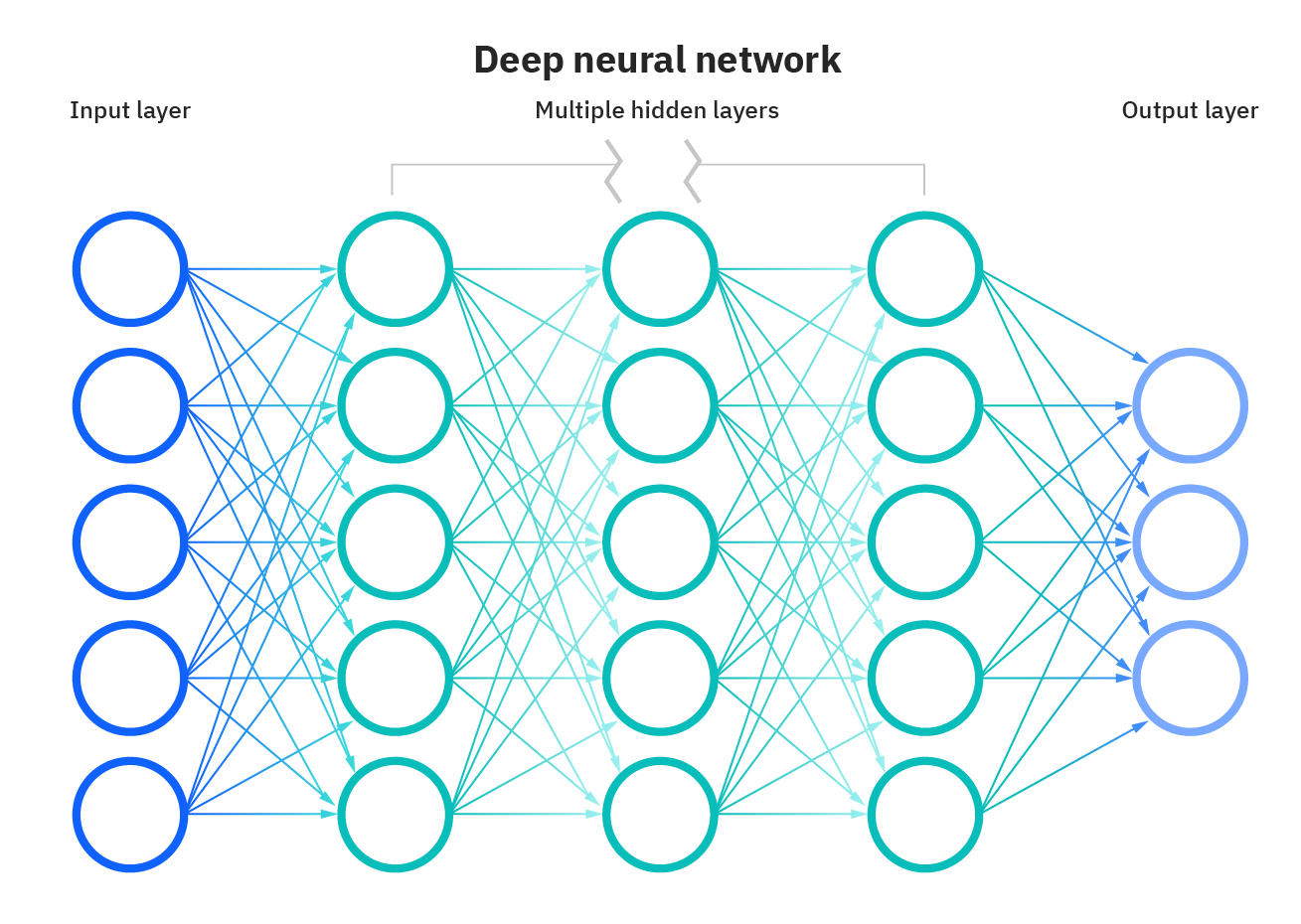
Models not only store architectural information (what types of layers and function are applied at every stage at inference), but weights as well. In the example of a neural network, each neuron stores weights and a bias.
\[\sum_{i=1}^{n} w_i x_i + b\]In the equation, $n$ is the total number of feature inputs that a neuron gets, $w_i$ is the weight associated with the feature input $i$, and $b$ is the bias term.
For each fully connected layer of a neural network, with $n_{\text{in}}$ neurons in the previous layer and $n_{\text{out}}$ neurons in the current layer, the size of the weight matrix between these layers are:
\[\text{Size of } W = n_{\text{in}} \times n_{\text{out}}\]The size of the bias terms is just the number of neurons in the current layer or:
\[\text{Size of } B = n_{\text{out}}\]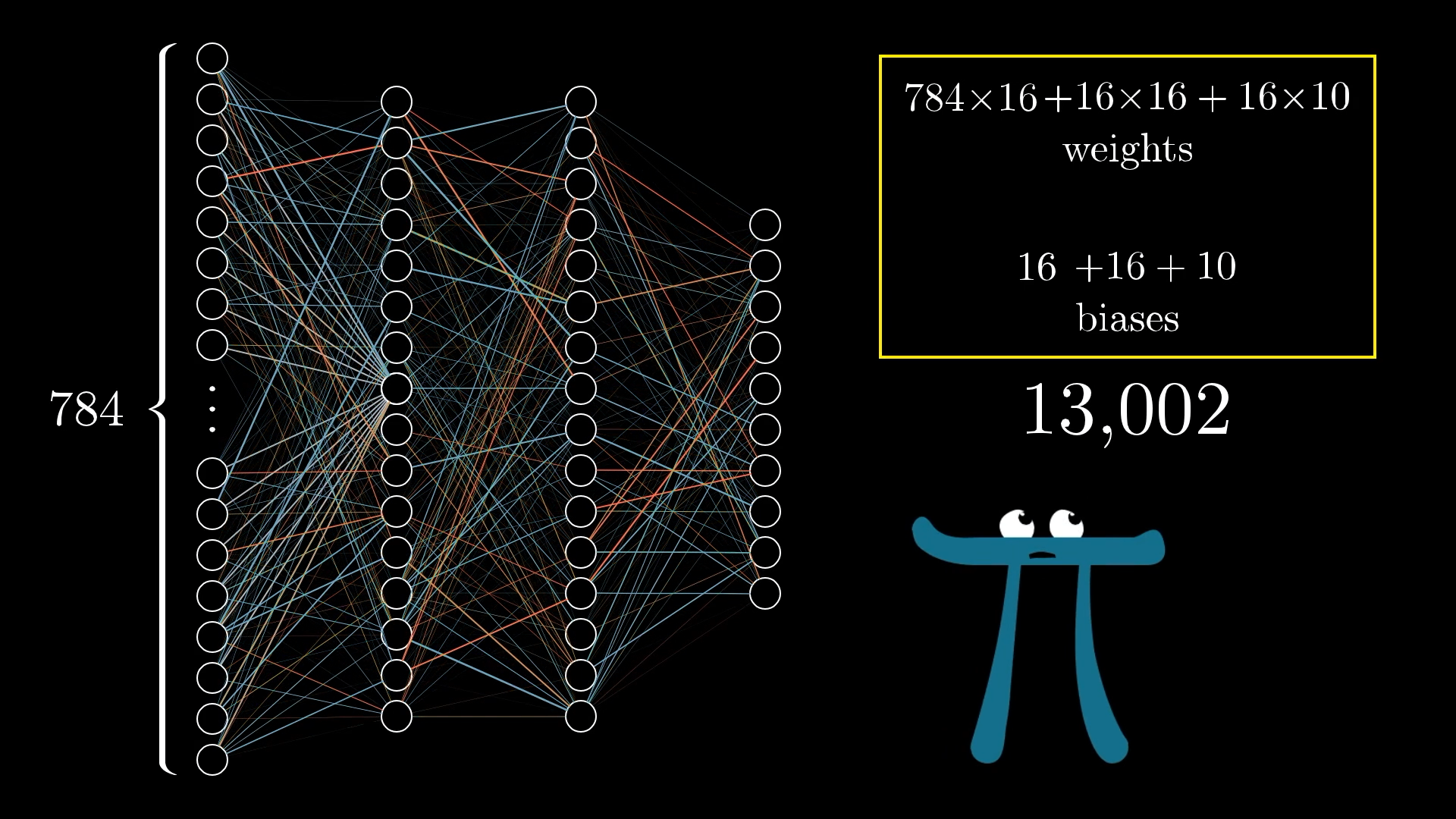 https://www.3blue1brown.com/lessons/neural-networks#more-neurons
We can represent the total number of parameters (weights and biases) of the model using this equation:
\[\text{# of Parameters} = \sum_{i=1}^{L-1} (n_i * n_{i+1} + n_{i+1})\]Where $L$ is the number of fully connected layers in the neural network and $n_i$ is the number of neurons in layer $i$.
The total Model Size is given in this equation (given the whole neural network uses the same data type)
\[\text{Model Size} = \text{# of Parameters} *\text{Bit Width}\]We will explore how to reduce both Number of Parameters (using Pruning) and Bit Width (using Quantization)
Model Speed
Unlike model size, model speed can be much more variable. Model speed depends on hardware, software, and other external factors like power.
To try to isolate the model performance to be agnostic to these factors, we use the number of mathmatical operation that a model uses, also called OPs, to generalize performance metrics. To measure how well the hardware works (or how well the model performs on specific hardware), we time these OPs and call them OPS or operations per second (note the capitalization). Most operations that happen in a neural network usally involve two OPs, multiply weights and add bias. This is often referenced as a MAC (Multiply-Accumulate Operation).
We mentioned before that another metric used is FLOPs or floating point operations per second. Since floating point math requires more complex operations compared to interger calculations and models often use floating point numbers, this is another important metric to measure the speed of a model.
Techniques for Smaller, Faster Models
There are a couple of different techniques to make smaller and more efficient ML models.
- pruning
- quantization
- knowledge distillation
- neural architecture search
- model/hardware specific optimizations
We will be looking only at the first 3 in this article, so that this explainer is more model agnostic.
Pruning
Pruning is a way to reduce the amount of redundant model weights and activations. It turns a model from a dense representation into a sparse representation while still trying to keep the model accurate.
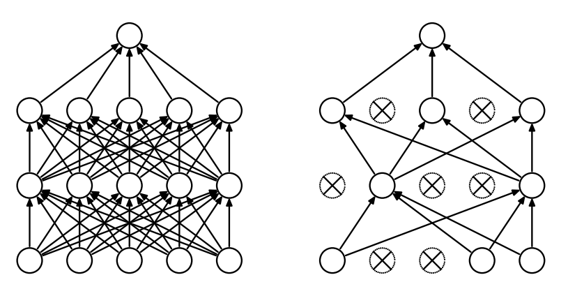
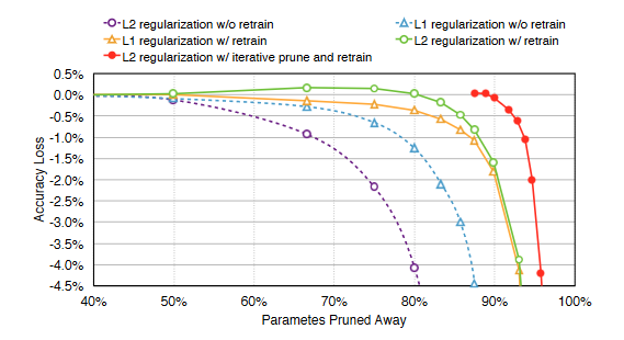
Pruning also happens in the human brain. A child has a large number of synapses per neuron, but as they get older, they start to reduce the number of synapses in their brain. Just pruning model weights themselves have a bad effect on accuracy, because you are just removing information that the model relies on to make predictions. When you prune and finetune the model, the reduced number of neurons can converge into a more sparse and less overfit representation of the data. This can lead to the same or even better performance compared to the original model. You can iteratively prune and finetune to refine the model even further, but there is diminishing return.
 https://arxiv.org/pdf/1506.02626
Pruning reduces the model size by on average around 10x but this effect can be compounded when also applying quantization.
Quantization
Quantization is the process of making models go from the continuous domain into the discrete domain to save model size and faster inference. We know that numbers in computers are stored in 1s and 0s, or bits. The way we can speed up model inference and shrink model sizes is to represent numbers in a model with the least amount of bits as possible. Not only are smaller bit numbers faster to compute and take less energy, they take up less memory meaning that the cache of processors can be utilized more effectively without having to load from RAM which can be very slow.
There are two parts to represent a floating point number in bits, a fractional part and an exponent part. The fractional part, also known as a mantissa, gives the number representation high precision while the exponent part gives the number high dynamic range. A similar example is when representing scientific numbers in the form $a*10^b$; a is a number between 0 and 10, representing the fractional (or linear) part, while b represents an exponent part which gives the number the ability to reach super high or low ranges. Different numerical representations trade off how many numbers are allocated to precision and how many are stored for high dynamic range.
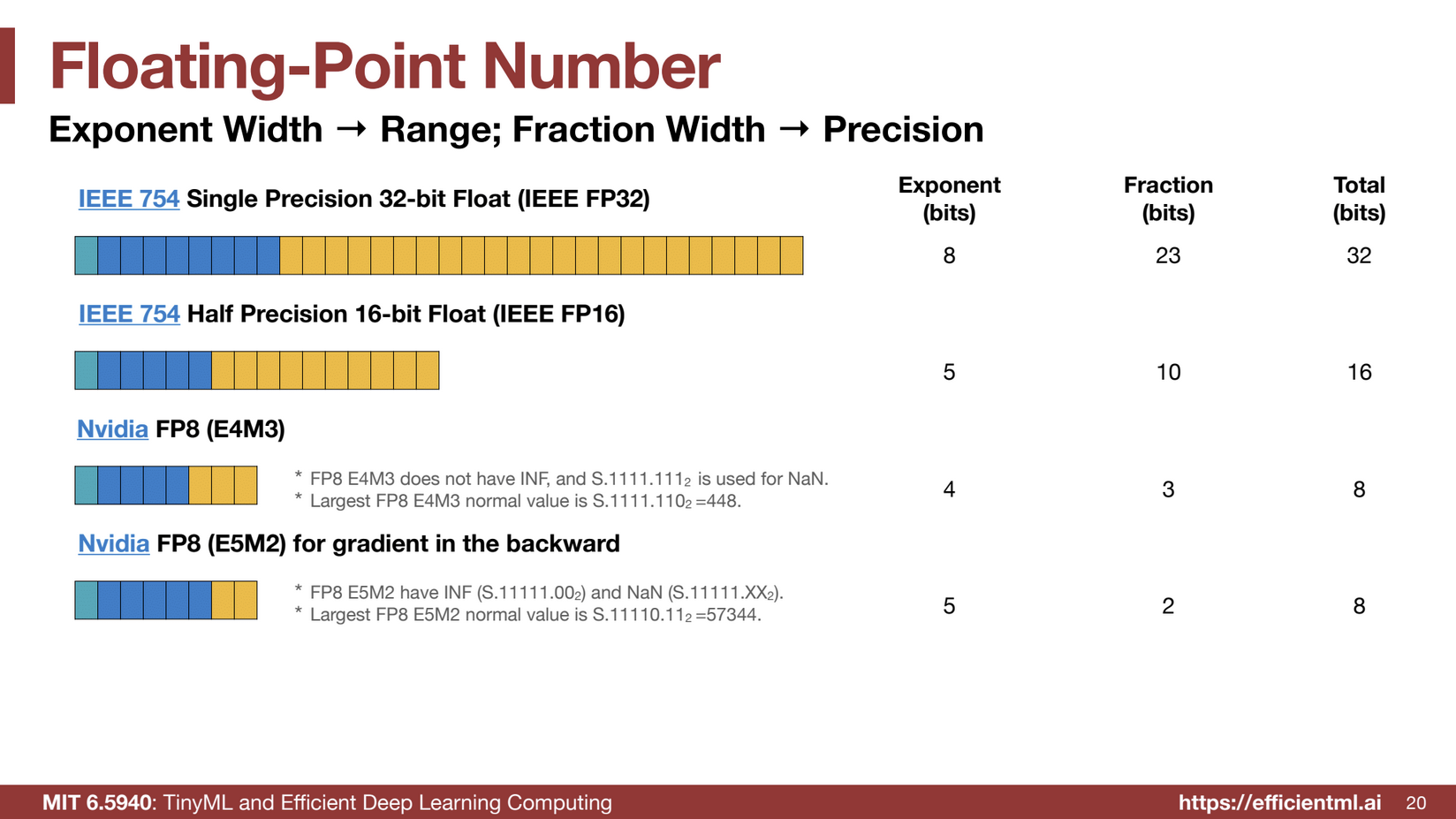 Commonly used floating point numbers for efficient storage
By specifying how these numbers are represented, it is possible to reduce the number of bits that are used, while keeping the numbers contained within weights to be similar to the original.
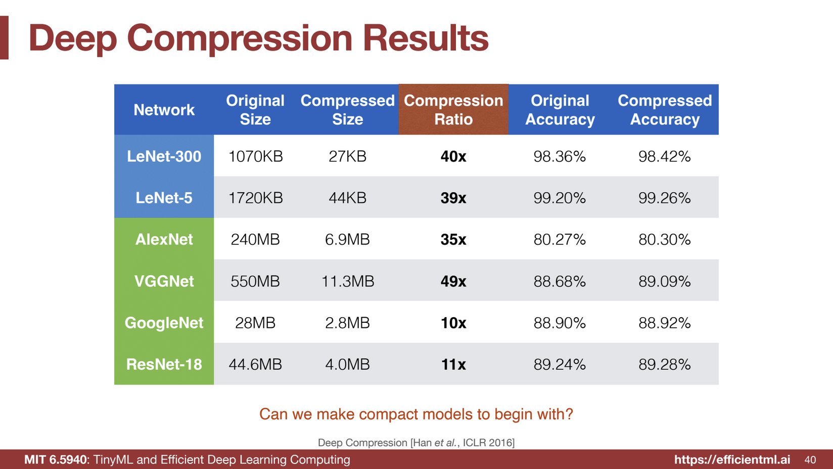
With Quantization, you can reduce the model size by around 30x, without sacrificing any accuracy (and often achieving higher accuracy).
Knowledge Distillation
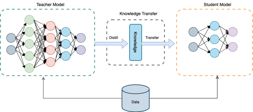
Knowledge Distillation is a technique where a larger, more complex model called the teacher model transfers its knowledge to the student model that is smaller and less complex. Instead of training a smaller model on the dataset where it is unlikely to get much performance because of its lack of complexity, it learns to replicate/mimic the larger model’s behaviors when looking at the same data.
There are a couple different ways to apply this technique:
- Minimize difference of output labels
- Minimize difference of class probabilities
- Minimize difference of logits
- Minimize difference of weights
- Minimize difference of sparsity
- Utilize TAs in support of Knowledge Distillation
I can’t go into the technical details of all of these techniques, but I will quickly discuss #2.
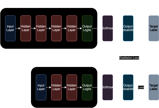
One of the ways to minimize the difference between the models is to minimize the difference of output probabilities. This way we can not only describe to the student model what is the right or wrong answer but also the relationship of the classes in regards to the output. For example, if there were 10 classes of animals and the model was fed a picture of a lion, the lion’s probabilities would be more similar to the probability of a deer compared to the probability of a fish. We would like the student to capture not only the correct classification of animals, but also the relationships between classes as a way to speed up learning.
Fun Fact: This Knowledge Distillation/Knowledge Transfer Framework was developed in the early days at Microsoft for their Xbox Kinect platform for doing human pose estimation.
Create our own small model (Demo)
Problems with Practical On-device ML
Prompt injections were popular ways of exploiting models in the early stages of the release of LLMs, since it was difficult to catch all edge cases, but many exploits of this kind are patched in more advanced systems through filtering. This is still an unsolved problem with on-devices systems, since all the information about the model is on-device.
So how is this a problem with on-device models now?
LLMs take in some meta tokens during training to indicate things like the start/end of a string input. If a user is able to find these meta tokens used in training, they are able to inject a prompt between meta tags to ignore instructions specified by the original meta tags. It would be nearly impossible to find these meta tags if they were stored in a secured server, but since all parts of the inference pipeline are stored locally, encrypted files can be unencrypted (since the model needs to unencrypt them to run), exposing them to the user. These meta tags can be then used in the user’s instructions to ignore all previous instructions created by the author of the model. A great demonstration of this is shown in this video by Evan Zhou.
Resources
Here are some extra resources I learned from if you want to dive deeper into the topic: